In this post, we will talk about what is the tensor, how it is stored in memory, and what reshaping operations we can apply on tensors.

Tensors

The tensor is the central data structure in Pytorch. Tensor is an n-dimensional data structure that contains some data in scalar type. Some of the types are boolean, integer and float. Imagine tensor as consisting of some data and some metadata describing its size/dimension, data type and where it is stored.

Tensor Stride/Storage

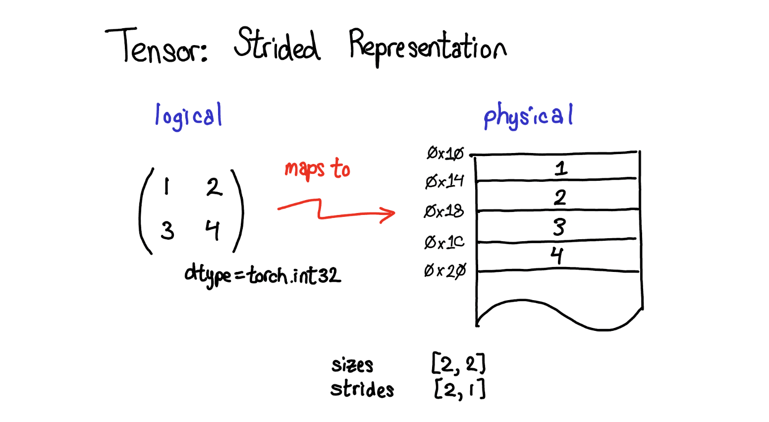
We can imagine tensor as a combination of two parts: logical and physical. Logical part is how we represent it, physical part is how it is actually stored on our computersThe most common physical representation is to lay out each element of the tensor contigously in the memory. For example, in the example below, the tensor contains 32-bit integers,each integer lies int he physical address, each offset four bytes from each other. Tensor Representation .

The lay out of the tensor in the physical representaiton is stored in layout field of Tensor object. Some of the popular layouts are strided, sparse, etc. In this post, I will only talk about strided layout to just give one example in action.

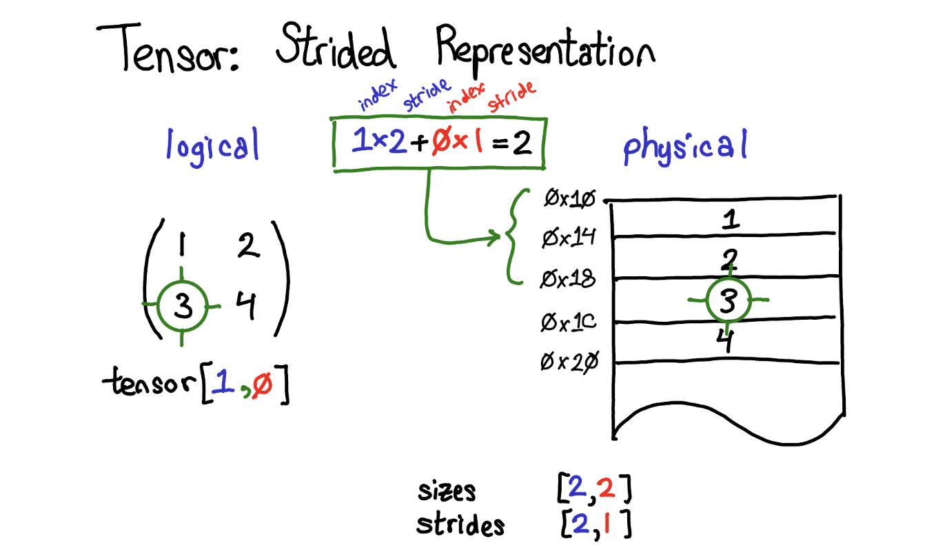
Strides helps us to translate logical view to physical view. In other words, if you want to read any particular element(s) of your tensor (ex: tensor[2,3]), stride helps you how to find this element in the physical storage (memory). Stride is the jump necessary to go from one element to the next one in the specified dimension. A tuple of all strides is returned when no argument is passed in. Otherwise, an integer value is returned as the stride in the particular dimension. They basically tell us, how many “steps” we skip in memory to move to the next position along a certain axis.

>>> t= torch.tensor([[1,1,1,1],
...                  [2,2,2,2],
...                  [3,3,3,3]], dtype=torch.int32)
>>> t.stride()
(4, 1)
>>> t.stride(0)
4
>>> t.stride(1)
1
>>> t.shape
torch.Size([3, 4])

In the example above, our first dimension is row, second dimension is column. So, (4,1) means that, to reach to the next row, you have to skip 4 elements, to reach to the next column, you have to skip one elements(basically next element). And, if you want to find a particular element in the memory, you multiple each index with the respective stride for that dimension and sum them al together. Check the example in the image below. logical-to-physical

Contigous() vs non-contigous()

A contiguous tensor is a tensor whose elements are stored in a contiguous order without leaving any empty space between them. A tensor created originally is always a contiguous tensor.Now, lets play with a contigous tensor, and make it non-contigous and see how stride is getting affected by this and why.

>>> # Create a tensor of shape [4, 3]
>>> x = torch.arange(12).view(4, 3)
>>> x
tensor([[ 0,  1,  2],
        [ 3,  4,  5],
        [ 6,  7,  8],
        [ 9, 10, 11]])
>>> x.stride()
(3, 1)
>>> x.is_contiguous()
True

If we look at the strides, we see, that we would have to skip 3 values to go to the new row, while only 1 to go to the next column. That makes sense so far. The values are stored sequentially in memory, i.e. the memory cells should hold the data as [0, 1, 2, 3, …, 11].

Now lets transpose the tensor, and have again a look at the strides:

>>> y = x.t()
>>> y
tensor([[ 0,  3,  6,  9],
        [ 1,  4,  7, 10],
        [ 2,  5,  8, 11]])
>>> y.stride()
(1, 3)
>>> y.is_contiguous()
False

First of all, getting transpose of contiguous tensor, makes it non-contiguous. However, the strides are now swapped. In order to go to the next row, we only have to skip 1 value, while 3 to move to the next column. This makes sense, if we recall the memory layout of the tensor:[0, 1, 2, 3, 4, …, 11] In order to move to the next column (e.g. from 0 to 3, we would have to skip 3 values. The tensor is thus non-contiguous anymore!

Now, lets make the tensor contigous, again.

>>> y = y.contiguous()
>>> y.stride()
(4, 1)
>>> y.is_contiguous()
True

If you call contiguous() on a non-contiguous tensor, a copy will be performed. Otherwise it will be a no-op.

ReShaping Operations on Tensors

Reshaping operations are probably the most important type of tensor operations. Reshaping allows us to change the shape with the same data and number of elements as self but with the specified shape, which means it returns the same data as the specified array, but with different specified dimension sizes

ReShape

Reshape method of tensor returns a tensor with the same data and number of elements as self, but with the specified shape. When possible, the returned tensor will be a view of input. Otherwise, it will be a copy. Contiguous inputs and inputs with compatible strides can be reshaped without copying.

>>> t=torch.arange(12)
>>> t
tensor([ 0,  1,  2,  3,  4,  5,  6,  7,  8,  9, 10, 11])
>>> a=t.reshape(2,6)
>>> a
tensor([[ 0,  1,  2,  3,  4,  5],
        [ 6,  7,  8,  9, 10, 11]])
>>> t
tensor([ 0,  1,  2,  3,  4,  5,  6,  7,  8,  9, 10, 11])
>>> a.storage().data_ptr()
140697029066880
>>> t.storage().data_ptr()
140697029066880
>>> torch.equal(a,t)
False
>>> a.reshape(-1)
tensor([ 0,  1,  2,  3,  4,  5,  6,  7,  8,  9, 10, 11])
>>> a
tensor([[ 0,  1,  2,  3,  4,  5],
        [ 6,  7,  8,  9, 10, 11]])

View

A view of a tensor returns a new tensor with the same data as the self tensor but of a different shape. The returned tensor shares the same data and must have the same number of elements, but may have a different size. For a tensor to be viewed, the new view size must be compatible with its original size and stride

>>> x=torch.rand(4,4)
>>> x
tensor([[0.3314, 0.9901, 0.5824, 0.3573],
        [0.2186, 0.5349, 0.4808, 0.6877],
        [0.3436, 0.0815, 0.0949, 0.0022],
        [0.3279, 0.2055, 0.6683, 0.1962]])
>>>
>>> y=x.view(16)
>>> y
tensor([0.3314, 0.9901, 0.5824, 0.3573, 0.2186, 0.5349, 0.4808, 0.6877, 0.3436,
        0.0815, 0.0949, 0.0022, 0.3279, 0.2055, 0.6683, 0.1962])
>>> z = x.view(-1, 8)
>>> z
tensor([[0.3314, 0.9901, 0.5824, 0.3573, 0.2186, 0.5349, 0.4808, 0.6877],
        [0.3436, 0.0815, 0.0949, 0.0022, 0.3279, 0.2055, 0.6683, 0.1962]])

One of the interesting feature of view, is ability to convert between dtypes
view(dtype) → Tensor

Returns a new tensor with the same data as the self tensor but of a different dtype.

If the element size of dtype is different than that of self.dtype, then the size of the last dimension of the output will be scaled proportionally. For instance, if dtype element size is twice that of self.dtype, then each pair of elements in the last dimension of self will be combined, and the size of the last dimension of the output will be half that of self. If dtype element size is half that of self.dtype, then each element in the last dimension of self will be split in two, and the size of the last dimension of the output will be double that of self

>>> a=torch.rand(2,2)
>>> a
tensor([[0.9259, 0.7836],
        [0.1964, 0.1979]])
>>> a.dtype
torch.float32
>>> a.view(torch.int32)
tensor([[1064110094, 1061722456],
        [1044976504, 1045081164]], dtype=torch.int32)
>>> a.view(torch.int16)
tensor([[  2062,  16237, -26280,  16200],
        [  4984,  15945, -21428,  15946]], dtype=torch.int16)

The Difference Between Tensor.view() and torch.reshape()

Both of pytorch tensor.view() and torch.reshape() can change the size of a tensor. What’s the difference between them?
tensor.view() must be used in a contiguous tensor, however, torch.reshape() can be used on any kinds of tensor

Ex: View can not run on non-contiguous tensor

>>> x = torch.tensor([[1, 2, 2],[2, 1, 3]])
>>> x = x.transpose(0, 1)
>>> x
tensor([[1, 2],
        [2, 1],
        [2, 3]])
>>> x.is_contiguous()
False
>>> y = x.view(3,2)
>>> y
tensor([[1, 2],
        [2, 1],
        [2, 3]])
>>> x.is_contiguous()
False
>>> y = x.view(2,3)
Traceback (most recent call last):
  File "<stdin>", line 1, in <module>
RuntimeError: view size is not compatible with input tensor's size and stride (at least one dimension spans across two contiguous subspaces). Use .reshape(...) instead.

However, reshape can run on non-contiguous tensor

>>> x = torch.tensor([[1, 2, 2],[2, 1, 3]])
>>> x = x.transpose(0, 1)
>>> x
tensor([[1, 2],
        [2, 1],
        [2, 3]])
>>> x.is_contiguous()
False
>>> y=x.reshape(2,3)
>>> y
tensor([[1, 2, 2],
        [1, 2, 3]])

Squeezing and Unsquezzing

The next way we can change the shape of our tensors is by squeezing and unsqueezing them.

Squeezing a tensor removes the dimensions or axes that have a length of one.
Unsqueezing a tensor adds a dimension with a length of one.

These functions allow us to expand or shrink the rank (number of dimensions) of our tensor.

>>> x=torch.arange(6)
>>> x
tensor([0, 1, 2, 3, 4, 5])
>>> x.unsqueeze(0)
tensor([[0, 1, 2, 3, 4, 5]])
>>> x.unsqueeze(1)
tensor([[0],
        [1],
        [2],
        [3],
        [4],
        [5]])


>>> x=torch.arange(6)
>>> x.reshape(2,3)
tensor([[0, 1, 2],
        [3, 4, 5]])
>>> x.squeeze()
tensor([0, 1, 2, 3, 4, 5])
>>> x.reshape(2,3)
tensor([[0, 1, 2],
        [3, 4, 5]])
>>> x.unsqueeze()
Traceback (most recent call last):
  File "<stdin>", line 1, in <module>
TypeError: unsqueeze() missing 1 required positional arguments: "dim"

Flatten

A flatten operation on a tensor reshapes the tensor to have a shape that is equal to the number of elements contained in the tensor. This is the same thing as a 1d-array of elements.

Flattening a tensor means to remove all of the dimensions except for one. The following is the representation of flatten method using methods mentioned above

def flatten(t):
    t = t.reshape(1, -1)
    t = t.squeeze()
    return t

Lets see in action:

>>> x=torch.zeros(2,2)
>>> x
tensor([[0., 0.],
        [0., 0.]])
>>> x=x.reshape(1,-1)
>>> x
tensor([[0., 0., 0., 0.]])
>>> x=x.squeeze()
>>> x
tensor([0., 0., 0., 0.])

Resources

http://blog.ezyang.com/2019/05/pytorch-internals/
https://pytorch.org/tutorials/beginner/basics/tensorqs_tutorial.html
https://deeplizard.com/learn/video/fCVuiW9AFzY
https://discuss.pytorch.org/t/contigious-vs-non-contigious-tensor/30107/2